Observability-aware Trajectories
The robotics problem of moving between two points typically wants to minimize distance travelled. What if we wanted the robot to move in a way that allows it to localize better? What would trajectories look like? Use the interactive diagram below to find out.
Abstract—Many trajectory generation schemes exist to find shortest paths between two points, but these trajectories might leave robot states unobservable to the state estimator. In the interest of online self-calibration of robots, the question of how to model measurements to find the calibration parameters has seen a surge of interest. With that surge comes the question of how the robot should move in order to get the desired measurements for the models. We will look at one such scheme that addresses the problem through tools from dynamical systems formulated by
Introduction and Related Work
State estimation is a vital component of an autonomous system for its control. To tell a robot where to go, the controller must know where the robot is. State estimation algorithms use sensor measurements and interpret them through models to determine robot state. Sensors have their own set of states which must be known to use in the estimator's sensor model. These states are typically determined in a separate procedure outside of normal robot operation. For robots that want to autonomously operate for long periods of time, sensor degradation makes it necessary to recalibrate. The robot may be programmed to perform a standalone calibration routine, where it temporarily stops performing its primary task in order to calibrate itself. However, this downtime may be undesirable that want to maximize utilization of the robot such as in environmental monitoring, manufacturing, or transportation. Thus, being able to calibrate while operating would allow a robot to be more available for its designed task.
A problem of great research interest has been how to find calibration parameters such as the focal parameters of a camera, the wheel radius of a tire instrumented for odometry, or the angles between axes of an accelerometer.
An approach to calibration is the use of fiducial targets in an environment designed to find the calibration parameters in what is known as target-based calibration
Target-free calibration methods like in
Typical system decompositions of robot functionality decouples the tasks of state estimation and trajectory generation
Observability-aware trajectories are trajectories which are designed to render states more observable. Observability is a property from the field of dynamical systems which decides whether the inputs and outputs of a dynamical system are enough to determine its state.
By using this property, a trajectory generator can discern which trajectories will lead to higher accuracy state estimation.
We will look at how observability is incorporated into trajectory generation for the specific problem of a robot whose mission is to safely move between two positions. This will require deriving a cost function, and parametrization of the trajectory which will be used by an optimizer.
This cost function extends a different cost function originally used for the deployment problem by
Observability-aware Trajectory Generation Framework
In general, a trajectory generator seeks to find a safe collision-free trajectory to achieve some mission. In our discussion we will consider the mission of travelling between two points in the environment. For these missions, the trajectory generator is given a start position \(p_{\mathrm{start}}\) and goal position \(p_{\mathrm{goal}}\). We will look at how trajectories can be generated that give us a path from \(p_{\mathrm{start}}\) to \(p_{\mathrm{goal}}\) which makes calibration states more observable. This trajectory generation method given by Preiss et al.
Problem Setup
System Equations
We will consider systems of the form $$ \begin{aligned} \dot{\mathbf{x}} &= f(\mathbf{x}, \mathbf{u}) \\ \mathbf{z} &= h(\mathbf{x}) \end{aligned} $$ where \(\mathbf{x}\) are the states of the system, \(\mathbf{u}\) are the control inputs, and \(\mathbf{z}\) are the measurements. The function \(f\) is the dynamics model of the system describing how the system evolves over time, and \(h\) is the measurement function relating states to measurements. If a state is not affected by the dynamics of the system, and is not affected by other states or the inputs then it is a self-calibration state \(\mathbf{x}_{sc}\).
Environment
The environment we are planning in consists of convex polytopes \(\mathcal{P}_1, \mathcal{P}_2, \ldots, \mathcal{P}_n\) defined through half-plane constraints where each \(\mathcal{P}_i = \{ \mathbf{y} \in \mathbb{R}^k | \mathbf{A}_i\mathbf{y}\leq \mathbf{b}_i \} \). We will require that each adjacent polytope overlaps by constraining \(\mathcal{P}_i \cap \mathcal{P}_{i+1} \neq \emptyset\) and that \(p_{\mathrm{start}} \in \mathcal{P}_1\), \(p_{\mathrm{goal}} \in \mathcal{P}_n\) to ensure that a path exists. The polytopes do not need to be bounded, but it is assumed that a higher level planner provides a perfect polytope representation of the environment a priori.
Nonlinear Observability
A system is considered observable if the initial state can be determined from the inputs and outputs of the system. For nonlinear systems, there is a distinction between systems that are globally observable and weakly locally observable. If no two initial conditions \(\mathbf{x}_0(0)\) and \(\mathbf{x}_1(0)\) along with control input \(\mathbf{u}(t)\) have the same output \(\mathbf{z}(t)\), then the system is called globally observable. A system may not be globally observable, but still weakly locally observable if there are no two initial conditions \(\mathbf{x}_0(0)\) and \(\mathbf{x}_1(0)\) in the same neighbourhood that have the same output \(\mathbf{z}\)
There is a test using the nonlinear observability matrix which determines whether or not a nonlinear system is weakly locally observable.
Nonlinear Observability Test
The \(i\)-th Lie derivative of a sensor model \(\mathbf{L}_i^h\) is defined through a recurrence relation. The \(0\)-th Lie derivative is given by the sensor model $$ \mathbf{L}_0^h = h(\mathbf{x}) $$ and the consecutive Lie derivative is found through $$ \begin{aligned} \mathbf{L}_{i+1}^h &= \frac{\partial}{\partial t} \mathbf{L}_i^h \\[2ex] &= \frac{\partial}{\partial t} \mathbf{L}_i^h \\[2ex] &= \frac{\partial h}{\partial\mathbf{x}} \frac{\partial\mathbf{x}}{\partial t} \\[2ex] &= \frac{\partial \mathbf{L}_i^h}{\partial \mathbf{x}} f(\mathbf{x}, \mathbf{u}). \end{aligned} $$ We denote the state derivative of the \(i\)-th Lie derivative by $$ \nabla \mathbf{L}_i^h = \frac{\partial \mathbf{L}_i^h}{\mathbf{x}} $$ and use it to construct the nonlinear observability matrix: $$ \mathbf{O}(\mathbf{x}, \mathbf{u})= \begin{bmatrix} \nabla \mathbf{L}_0^h \\[1ex] \nabla \mathbf{L}_1^h \\[1ex] \vdots \\[1ex] \nabla \mathbf{L}_k^h \end{bmatrix} $$ which has full column rank for some \(k\) if and only if the system is weakly locally observable. While this property is informative, it only tells us whether the system is observable, or not observable. In order to generate an objective function for observability, we need a metric of how well observable a system is.
Observability Quality Metric
Linear Algebra Preliminaries
We will review basic properties of matrices that are used to formulate a observability quality metric. Let \(\mathbf{A}\) be an \(m \times n\) matrix. The null space of \(\mathbf{A}\) is \(\mathrm{Null}(\mathbf{A}) = \{\mathbf{x} \in \mathbb{R}^n \,|\,\mathbf{Ax} = \mathbf{0} , \mathbf{x} \neq \mathbf{0}\}\), i.e., the set of non-trivial vectors \(\mathbf{x}\) which map to the zero vector \(\mathbf{0}\). If \(\mathrm{dim}(\mathrm{Null}(\mathbf{A})) > 0\), then the matrix is not full rank as a consequence by the Rank-Nullity theorem which states $$ \textrm{Rank}(\mathbf{A}) + \mathrm{dim(Null}(\mathbf{A})) = n. $$ Such a matrix with a non-empty null space is non-invertible and we say that \(\mathbf{A}\) is singular.
The singular value decomposition of a matrix \(\mathbf{A}=\mathbf{USV}\) results in three components: an orthonormal matrix, a diagonal matrix, and another orthonormal matrix. \(\mathbf{U}\) and \(\mathbf{V}\) are the orthonormal matrices and \(\mathbf{S}\) is a diagonal matrix giving the singular values of the matrix where $$ \mathbf{S} = \mathrm{diag}(\sigma_1, \sigma_2, \ldots,\sigma_n). $$ The singular values of a matrix can be used to determine its rank, and thus its singularity.
Lemma: If a matrix \(\mathbf{A}\) with \(\mathrm{Rank}(\mathbf{A}) = r\), then A has \(r\) non-zero singular values.
Corollary: If a matrix has one or more zero singular value, then the matrix is singular and thus has a non-empty null space.
Thus, the null space of a matrix gives us the values which the matrix maps to the zero vector. Moreso, the size of the null space can be determined through singular value decomposition through examination of the diagonal matrix \(\mathbf{S}\). These singular values of a matrix can be used to quality how close to singularity a matrix is, where the smallest singular value is the component closest to singularity.
Local Observability Gramian (LOG)
The use of the local observability Gramian to measure how well a system is observable was introduced by
The singular values of the LOG give the observability metric we seek for observability-aware trajectory generation. The element \([\mathbf{W_O}]_{i,j}\) gives the effect of state \(x_j\) on output \(z_i\). The \(j\)-th singular values of \(\mathbf{W_O}\) is a measure of the distance of the state \(x_j\) is from the unobservable subspace \(\mathcal{U}_O\). States which have larger singular values are more well observable, and states with the lowest singular values are the least observable. The smallest singular value is the observability of the least observable state and thus, the maximization of the smallest singular value of the LOG may be used as our cost function.
In practice, calculating the LOG is expensive due to the presence of the state transition matrix \(\mathbf{\Phi}(0, t)\) in the integral which may not have a closed form solution for many nonlinear systems. Approximations of the LOG whose null space has the same properties of quantifying observability quality must thus be made for use in an optimization framework.
Expanded Empirical Local Observability Gramian (E\(^2\)LOG)
The E\(^2\)LOG avoids the expensive calculation of the state transition matrix by using an approximation of the sensor model Jacobian, which is denoted as \(K_{t_0}(t) = \frac{\partial}{\partial \mathbf{x}}h(t)\) obtained by Taylor expansion of \(h(t)\) around time \(t_0\):
$$
\begin{aligned}
h_{t_0}(t)
&= h_{t_0}(\mathbf{x}(t), \mathbf{u}(t)) \\[2ex]
&= \sum_{i=0}^n \frac{(t-t_0)^i}{i!}\frac{\partial ^ i}{\partial t^i}h\left(\mathbf{x}(t_0), \mathbf{u}(t_0)\right) \\[2ex]
&=\sum_{i=0}^n \frac{(t-t_0)^i}{i!} \mathbf{L}_h^i(\mathbf{x}(t_0), \mathbf{u}(t_0)),
\end{aligned}
$$
and differentiating it with respect to the state to obtain
$$
\begin{aligned}
K_{t_0}(t)
&= \frac{\partial}{\partial \mathbf{x}}h_{t_0}(t) \\[2ex]
&= \frac{\partial}{\partial \mathbf{x}}\sum_{i=0}^n \frac{(t-t_0)^i}{i!} \mathbf{L}_h^i(\mathbf{x}(t_0), \mathbf{u}(t_0)) \\[2ex]
&= \sum_{i=0}^n \frac{(t-t_0)^i}{i!} \frac{\partial}{\partial \mathbf{x}}\mathbf{L}_h^i(\mathbf{x}(t_0), \mathbf{u}(t_0)) \\[2ex]
&= \sum_{i=0}^n \frac{(t-t_0)^i}{i!}\nabla \mathbf{L}_h^i(\mathbf{x}(t_0), \mathbf{u}(t_0)). \\[2ex]
\end{aligned}
$$
This Jacobian reveals the effects of states on outputs and is used to approximate the LOG in the Expanded Empirical Local Observability Gramian (E\(^2\)LOG) matrix:
$$
\mathbf{W_O}'(0,T,\Delta t) = \int_0^T K_t(t + \Delta t)^TK_t(t + \Delta t) dt,
$$
where the approximated Jacobian is evaluated some small time \(\Delta t\) ahead of the linearization point in order to incorporate states which do not directly appear in the measurement model. This accounting of system dynamics is made possible with the incorporation of higher-order Lie derivatives in the linearization, which was not previously done in another approximation
The \(E^2\)LOG is used in place of the LOG due to its relative ease of computation, and its singular values will be used as part of our optimization. The order of the Taylor expansion is dependent on the number of Lie derivatives required to make the system observable. Blocks of the E\(^2\)LOG can be narrowed to incorporate only the self-calibration states \(\mathbf{x}_{sc}\) whose observability we want to improve in the trajectory. Its computation doesn't include find a system's state transition matrix, which might not have an analytic solution. Thus, maximizing the smallest singular value of the E\(^2\)LOG gives trajectories that make the least observable state more observable.
Representing Trajectory
In order to formulate our problem as an optimization problem, a formal description of what the trajectory is and how to represent it is needed along with an optimizable trajectory parametrization that guarantees safe, collision-free trajectories.
Differentially Flat Systems
For trajectory representation, we look at the notion of differentially flat outputs of a system to represent trajectories as in
Bézier Curves
For simplicity in optimization, the trajectory \(\mathbf{y}(t)\) is as a piecewise \(k\)-piece, degree-\(d\) polynomial and to guarantee collision-free paths assuming a perfectly known environment, the polynomials will be represented by a Bézier curve . A Bézier curve is a degree-\(d\) polynomial defined by \(d+1\) control points \(\mathbf{y}_i \in \mathbb{R}^k\) such that $$ f(\tau) = b_{0,d}(\tau)\mathbf{y}_0 + b_{1,d}(\tau)\mathbf{y}_1 + \cdots + b_{d,d}(\tau)\mathbf{y}_d, $$ for \(\tau \in [0,1]\) and where $$ b_{i,j}(\tau) = {j \choose i}\tau^i(1-\tau)^{j-i}, \quad i=0,1,\ldots,n. $$ The Bézier curve has the property that it is constrained to the convex hull of its control points as in the figure above. Thus by placing a Bézier curve inside each polytope and adding constraints to the control points that they satisfy the half-plane constraints will guarantee collision-free trajectories.
Optimization Objective
With the tools to quantify the quality of observability and represent the trajectory, the objective function which will be used to generate observability-aware trajectories is $$ \begin{aligned} &\mathrm{arg\,max}_{\mathbf{y}(t)} \,\sigma_{\mathrm{min}}(\mathbf{W_O}(0,T,\Delta t)) \\ &\text{s.t.} \qquad \mathbf{A}_i\mathbf{y}_{i,k} \leq \mathbf{b}_i \\ \end{aligned} $$ where \(\sigma_{\text{min}}(\cdot)\) extracts the smallest singular value,\(\mathbf{y}_{i,k}\) is the \(k\)-th control point of the Bézier curve inside \(\mathcal{P}_i\). Additional constraints may be added as such as constraining the dynamics at the endpoints, enforcing maximum values on the inputs, and restrictions based on the physical limits of the system. Depending on the constraints and the degree of the Bézier curve, the problem may be solved directly through a linear solve or least squares. If nonlinear inequalities are present, the designers of the framework suggest the Sequential Quadratic Programming (SQP) method as an effective optimization tool.
External Results
The method has been trialed in simulation
Simulation
We implement the method of maximizing the smallest singular value of the E\(^2\)LOG on a scalar double integrator system, as well as the minimum snap trajectory proposed in
Simulation Setup
We have a scalar point robot with a global positioning system (GPS) and a laser rangefinder (LRF). The GPS provides absolute positions, but its measurements have low frequency and a large amount of noise compared to the LRF which gives higher frequency measurements with lower noise. The LRF measurements are affected by a multiplicative scale parameter which must be calibrated for. This setup reflects field setups where the low frequency and high noise of GPS are supplemented with another sensor using sensor fusion
System Equations
Our system has state vector \( \mathbf{x}=\begin{bmatrix}x && \dot{x} && s\end{bmatrix}^T \), where \(x\) is the system's position and \(s\) is the scale parameter of the LRF. We have a single input \(\mathbf{u} = \begin{bmatrix}\ddot{x}\end{bmatrix}\), and the measurements \(\mathbf{z} = \begin{bmatrix}z_{\text{GPS}} && z_{\text{LRF}}\end{bmatrix}^T\) corresponding to the range measurements of each of the sensors. Our system equations are: $$ \begin{aligned} \dot{\mathbf{x}} &= \begin{bmatrix} 0 && 1 && 0 \\ 0 && 0 && 0 \\ 0 && 0 && 0 \end{bmatrix} \mathbf{x} + \begin{bmatrix} 0 \\ 1 \\ 0 \end{bmatrix} \mathbf{u} \\[4ex] \mathbf{z} &= \begin{bmatrix} x\\ xs \end{bmatrix}, \end{aligned} $$ and we have a single self-calibration parameter of the range scale \(\mathbf{x}_{sc}=s\). We further constrain the system to be in \([0, 10]\) as our environment.
Observability Analysis
The system is observable given the test provided by the nonlinear observability matrix. Two Lie derivatives are needed to make the system observable: $$ \begin{aligned} \nabla {\mathbf{L}}_0^h &= \begin{bmatrix} 1 && 0 && 0\\ s && 0 && p \end{bmatrix}\\[2ex] \nabla {\mathbf{L}}_1^h &= \begin{bmatrix} 0 && 1 && 0\\ 0 && s && v \end{bmatrix}, \end{aligned} $$ resulting in the observability matrix $$ \mathbf{O}(\mathbf{x}, \mathbf{u}) = \begin{bmatrix} 1 && 0 && 0\\ s && 0 && p\\ 0 && 1 && 0\\ 0 && s && v \end{bmatrix} $$ Since \(\mathbf{O}(\mathbf{x}, \mathbf{u})\) has full column rank, the system is observable.
Differential Flatness
Following the example for the UAV experiment given by
Simulation Parameters
We chose hyperparameters for our experiment trying to match real world scenarios when possible. Our experiments have a ground truth value for the range scale of \(s=1.2\). The frequency of the LRF is 100 Hz, and its range measurements have a standard deviation of 0.02 m. The GPS has a frequency of 0.5 Hz, and its measurements have a standard deviation of 5 m which is realistic for GPS where the satellite signal is weak
Results
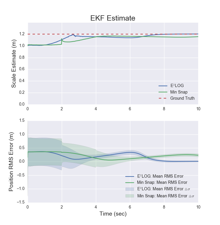
Below: Mean position error estimate and uncertainty with E\(^2\)LOG and Min Snap trajectories aggregated over 1000 trials.
The E\(^2\)LOG trajectory results in convergence to the ground truth of the scale estimate while the minimum snap trajectory does not. As a result, the final position error is lower in the E\(^2\)LOG trajectories than in the minimum snap trajectories. Between 3.8s and 6.4s, the position error for the E\(^2\)LOG trajectory is higher than the minimum snap trajectory. We suspect that the more aggressive maneuvers performed by the minimum snap trajectory resulted in larger errors accumulating in the update step of the EKF but have not yet determined the root cause.
| Errors accumulated over 1000 trials | E\(^2\)LOG | Minimum Snap |
|---|---|---|
| Final Mean Error (m) | 0.012 | 0.216 |
| Final Standard Deviation (m) | 0.021 | 0.055 |
| Integrated RMS Error (m) | 176.8 | 211.3 |
In our simulation, we see a 21x better final mean error and half the final standard deviation in position for the E\(^2\)LOG trajectory compared against the minimum snap trajectory. This greatly exceeds the 4x improvement seen by
Future Work
There are research problems still unanswered in the areas of observability analysis and trajectory generation. The inclusion of higher-order Lie derivatives motivated the formulation of the E\(^2\)LOG as opposed to the observability quality metric proposed in
In addition to the research problems, there are also extensions that could be made to our simulation. One possible extension of our work would be the extension of our simulation to describe complete three-dimensional motion in \(SO(3)\) since robots operate in this space. Also, our simulation could be extended to include multiple self-calibration states which would validate the multi-state scaling method described in
Conclusion
In conclusion, we have presented a framework which optimizes trajectories for observability of self-calibration states by maximizing the smallest singular value of an approximated observability Gramian. We validate the system in the simulation of a modified double integrator system with nonlinear measurements. We compared the results of the EKF state estimator's accuracy using trajectories that were observability-aware and a trajectories which had minimal snap. The simulation results show that the observability-aware trajectories achieve more accurate and confident state estimation over the minimum-snap trajectory.